Quickstart

Minimal steady-state run

from lww_transport import LWWConfig, LWW1DSimulator

cfg = LWWConfig(nx=86, n=72, exchange=True, verbose=True)
sim = LWW1DSimulator(cfg)

steady = sim.solve_steady_state(bias=0.0, max_iterations=200)
print(steady.converged, steady.iterations)
print(steady.current[-1])

sim.save_state(steady.state, "lww_output")

Configuration summary

LWWConfig is organized into grouped sections while preserving flat keyword arguments such as nx=... and exchange=...:

cfg = LWWConfig.standard_rtd().with_grid(86, 72).with_bias(0.08)
sim = LWW1DSimulator(cfg)
print(sim.config_summary({"mode": "steady"}))

CLI simulations print the same summary and write config_summary.txt to the output directory. Direct transient runs also save the summary when output_dir is supplied.

Plot device geometry

The geometry helper draws the double-barrier RTD potential profile from the active LWWConfig:

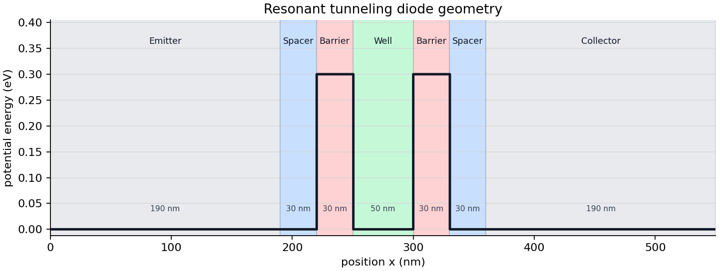
from lww_transport import LWWConfig, save_rtd_geometry_image

cfg = LWWConfig.standard_rtd()
save_rtd_geometry_image(cfg, "rtd_geometry.png")

The command line interface provides the same output:

lww-transport geometry --output output --nx 86 --n 72

Wigner phase-space image

The visualization module can draw a 3D Wigner phase-space surface with a contour projection and save the image directly. The example image below was generated from output_time_dependent/lww_pywigner.csv from a transient run:

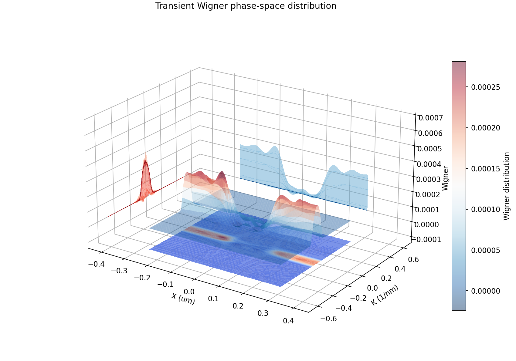
from lww_transport import (
    LWWConfig,
    LWW1DSimulator,
    save_wigner_phase_space_image,
)

cfg = LWWConfig(nx=86, n=72, exchange=True)
sim = LWW1DSimulator(cfg)
state = sim.initial_zero_bias_state()

save_wigner_phase_space_image(
    state.f,
    "wigner_phase_space.png",
    cfg=cfg,
    title="Zero-bias Wigner phase space",
    style="floating",
    surface_alpha=0.45,
    colorbar_label="Wigner distribution",
)

Saved state CSV files can be plotted without loading the simulator state manually:

save_wigner_phase_space_image(
    "lww_output/lww_pywigner.csv",
    "lww_output/wigner_phase_space.png",
    cfg=cfg,
)

Small-grid smoke run

The reference grid builds a large Wigner system. Smaller grids are appropriate for development checks:

cfg = LWWConfig(nx=10, n=8, exchange=False, verbose=True)
sim = LWW1DSimulator(cfg)

steady = sim.solve_steady_state(bias=0.0, max_iterations=20)
transient = sim.run_transient(
    steady.state,
    ivn=3,
    itn=30,
    dbias=0.008,
    sample_every=5,
    progress_every=5,
)

sim.save_transient(transient, "lww_output")

Profiling

Use the profiling helper to compare the C++, Numba, and Python assembly backends. All three paths use the same direct LAPACK banded solve; the backend choice controls matrix assembly and current/density reductions:

python scripts/profile_transient.py --nx 43 --n 36 --ivn 1 --itn 2 --backend cpp
python scripts/profile_transient.py --nx 43 --n 36 --ivn 1 --itn 2 --backend numba
python scripts/profile_transient.py --nx 43 --n 36 --ivn 1 --itn 2 --backend python

Legacy CSV output

save_state writes the following CSV files to the output directory:

• lww_pypoten.csv — electrostatic potential rvs

• lww_pydensity.csv — carrier density

• lww_pycurrent.csv — current density profile J(x)

• lww_pywigner.csv — Wigner distribution f (flattened)

• lww_pywigner_ss.csv — steady-state reference Wigner fr (flattened)

save_transient writes transient current traces named lww_tcurl_<bias>.csv, where <bias> is formatted to four decimal places (e.g. lww_tcurl_0.0080.csv).

When run_transient receives an output_dir value, it writes those lww_tcurl_<bias>.csv files incrementally every sample_every iterations. It also refreshes the state CSV checkpoint files after each completed bias point.