Notes on Probability Theory
Updated: 30 Jul 2025
Table of Content
- Table of Content
- Axiomatic Framework
- Events Relationship
- Random Variables and Their Distributions
- References
There are some jargons in probability that are worth knowing for they keep recurring in many fields of science. The idea of a function in relation to a probability is widespread used in complex systems, statistical mechanics, quantum mechanics, electromagnetism, and many more. So it is just logical to learn the jargons of probability so that next time it will not appear as wild beasts.
Axiomatic Framework
- probability space $(\Omega, \mathcal{F}, \mathcal{P})$:
- sample space $\Omega$, sometimes denoted by $S$ [2] or $U$ (universal set)
- a non-empty set of all possible elementary outcomes of a random experiment
- an outcome is the result of a single execution of the model, and one outcome is one point in the sample space
- depending on the nature of the experiment, it can be numbers, words,letters, or symbols
- can be categorized as: discrete sample spaces, continuous sample space
- properties of well-defined sample space: mutually exclusive outcomes, collectively exhaustive outcomes, appropriate granularity
- set of events $\mathcal{F}$: subset of the sample spcace to which probabilities can be assigned
- an event is a specific set of outcomes from the sample space
- “occurred” event $\in \mathcal{F}$
- set of all possible subsets of the sample space: $\mathcal{P}(\Omega)$, only sensible if you have discrete sample spaces but not on a continuous (uncountable) sample space
- to avoid problems-> restrict to a well-behaved collection of subsets, known as “measurable sets” to which we can assign probabilities
- the event space, must have a mathematical structure known as $\sigma$-algebra
- for continuous sample space like the real line $\mathbb{R}$, event space is the Borel $\sigma$-algebra $\mathcal{B}(\mathbb{R})$
- a probability measure $\mathcal{P}$: function that assigns a specific probability to each event
- its a real-valued function, $P : \mathcal{F} \to \mathbb{R}$, assigning each event $E \in \mathcal{F}$ to a number between 0 and 1, inclusive.
- what is a valid probability measure?
- it has to satisfy 3 fundamental axioms: kolmogorov’s axioms
- non-negativity: $P(E) \geq 0 $
- normalization: $P(\Omega)=1 $
- countable additivity (or $\sigma$-additivity): $P\left(\cup_{i=1}^{\infty} \right) = \sum_{i=1}^{\infty} P(E_i)$
- it has to satisfy 3 fundamental axioms: kolmogorov’s axioms
- the first 2 axioms are intuitive, the third axiom is the most profound and powerful
- consequences of the axioms: probability of empty set, probability of complement, addition law
- sample space $\Omega$, sometimes denoted by $S$ [2] or $U$ (universal set)
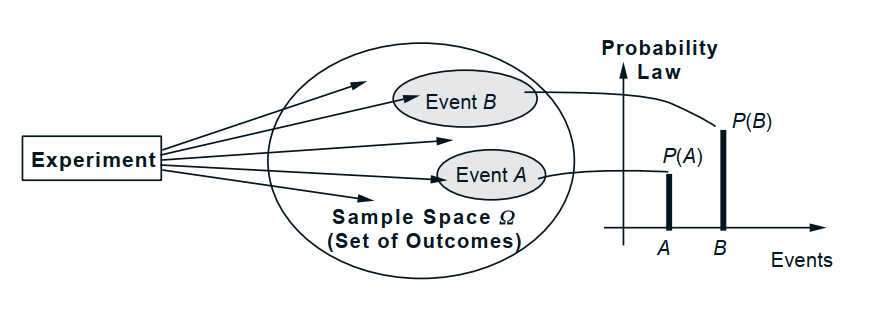
main ingredient of Probability Theory [3]
Events Relationship
- with the axiomatic framework of probability space in place, what are the concepts that describe the relationship between events?
Conditional Probability
- a measure of the probability of an event occurring, given that another event is already known, assumed, or asserted to have occurred
- the formal mathematical tool for updating our beliefs or assessments of likelihood in the face of new evidence
- core intuition behind conditional probability is the concept of reduced sample space
- ex: if event B has occurred, the set of all possible outcomes $\Omega$, is effectively reduced to the subset of outcomes contained within B, and any event outside of $B$ is no longer possible. Within this new smaller universe, we want to find the probability of another event $A$.
- the only outcome of $A$ that are still possible are those that are also in $B$
- outcomes in the $A \cap B$
- the only outcome of $A$ that are still possible are those that are also in $B$
- mathematical representation: ratio of the probability of their joint occurrence to the probability of the conditioning event
- the conditional probability of $A$ given $B$ -> $P(A | B)$
- definition: \begin{equation} P(A|B) = \frac{P(A\cap B)}{P(B)} \label{eq:conditional} \end{equation}
- ex: if event B has occurred, the set of all possible outcomes $\Omega$, is effectively reduced to the subset of outcomes contained within B, and any event outside of $B$ is no longer possible. Within this new smaller universe, we want to find the probability of another event $A$.
- core intuition behind conditional probability is the concept of reduced sample space
- rearranging equation (\ref{eq:conditional}) gives the multiplication rule: \begin{equation} P(A \cap B) = P( A | B) P(B) \end{equation}
Independence
- two events are statistically independent (or stochastically independent) if the occurrence of one event does not affect, alter, or provide any information about the probability of the other event occurring.
- the formal mathematical definition is based on the multiplication rule. \begin{equation} P(A \cap B) = P(B) P(A) \end{equation}
Mutual Exclusivity vs. Independence
- Mutually exclusive events: two events cannot happen at the same time $P(A\cap B) = 0$ since $A\cap B = \emptyset$.
- Independent events: two events are independent $P(A | B) = P(A)P(B)$
Random Variables and Their Distributions
Random Variable
- a variable that is subject to variations due to random chance. It is a result of a random experiment, a sampling. Since the variable is random you expect to get different values as you obtain multiple samples.
- conventionally denoted by capital letters: $X$, $Y$ [2],[3]
- formally, a function that assigns a real number to each elementary outcome in the sample space
- note: probability measure $\neq$ random variable
- outcome/event (x) -> random variable (X) -> probability measure $P({X=x}) = p_{X}(x)$
- note: probability measure $\neq$ random variable
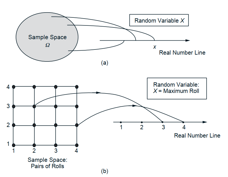
random variable mapping visualization[3]
- we can define a mean and variance to each random variable, we can conditioned it to another event, there is a notion of independece on random variable [3]
Distribution Function:
a function over a general set of values, also called as cumulative distribution function (CDF), or it may be referred to as a probability mass function (PMF). A probability distribution is a function that describes how likely you will obtain the different possible values of the random variable.
Probability Density Function
Density of a continuous random variable, is a function whose value at any given sample (or point) in the sample space (the set of possible values taken by the random variable) can be interpreted as providing a relative likelihood that the value of the random variable would equal that sample.
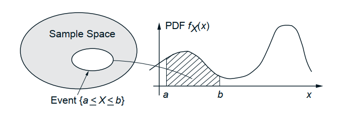
probability density function mapping [3]
PDF is used to specify the probability of the random variable falling within a particular range of values, as opposed to taking on any one value.
- Continuous Distribution:
\(Pr[a \leq X \leq b] = \int_a^b f_{X}(x) dx\)
“What is the probability that X falls between a and b?”
- Discrete Distribution:
\(f(t) = \sum p_i \delta (t - x_i)\)
Entropy
The entropy of a random variable is a function which attempts to characterize the “unpredictability” of a random variable. Its not about the number of possible outcome, it is also about their frequency. Thought, it sounds like a vague concept, it has a precise mathematical definition.
Take for example a random variable X with values \(X = \{x_1, x_2, ..., x_n\}\) and is defined by a probability distribution P(X), the entropy of the random variable is:
\[H(X) = -\sum P(x) \log P(x)\]Conditional Entropy
quantifies the amoutn of information needed to describe the outcome of a random variable Y given that the value of another random variable X is known.
Joint Entropy
The entropy of a joint probability distribution, or a multi-valued random variable. Joint entropy is a measure of the uncertainty associated with a set of variables.
The join Shannon entropy of two discrete random variables X and Y is defined as
\[H(X,Y) = - \sum_{x} \sum_{y} P(x,y) \log_{2} [P(x,y)]\]where x and y are particular values from X and Y and P(x,y) is the joint probability of these values occurring together.
Mutual Information (MI)
MI of two random variables is a measure of the mutual dependence between the two variables. Specifically quantifying the information content obtained about one random variable, through the other random variable. Thus it is linked to that of entropy of a random variable.
MI of two discrete random variables X and Y can be defined as: \(I(X;Y) = \sum_{y \in Y} \sum_{x \in X} p(x,y) \log \frac{p(x,y)}{p(x)p(y)}\)
MI of two continuous random variables X and Y can be defined as: \(I(X;Y) = \int_{Y} \int_{X} p(x,y) \log \frac{p(x,y)}{p(x)p(y)} dxdy\)
Note that if X and Y are independent, \(p(x,y)=p(x)p(y)\) therefore:
\[\log \frac{p(x,y)}{p(x)p(y)} = \log(1) = 0\]MI properties:
a. nonnegative: \(I(X;Y)\)
b. symmetric: \(I(X;Y)=I(Y;X)\))=
Relation to conditional and join entropy
\(1. I(X;Y) = H(X)-H(X\|Y)\) \(2. I(X;Y) = H(X,Y)-H(X\|Y)-H(Y\|X)\) \(3. I(X;Y) = H(X)+H(Y)-H(X,Y)\)
\(H(X),H(Y)\) = marginal entropies
\(H(X\|Y)\) = conditional entropies
\(H(X,Y)\) = joint entropies