Notes on the Art of Molecular Dynamic Simulations
Updated: 04 Aug 2025
author’s work:
- polymer chain dynamics, event-driven simulation for hard-sphere systems, the simulation of hydrodynamic phenomena like eddy formation, and the self-assembly of complex structures
Table of Content
Foundational Chapters (1-5)
code: https://github.com/antble/artofmd
chapter 1-2
- lays the conceptual groundwork
- principles of computer simulation as a bridge between microscopic interactiona dn macroscopic properties
- basic molecular dynamics
- simulation of a 2D soft-disk fluid: a system composed of purely repulsive spherical particles
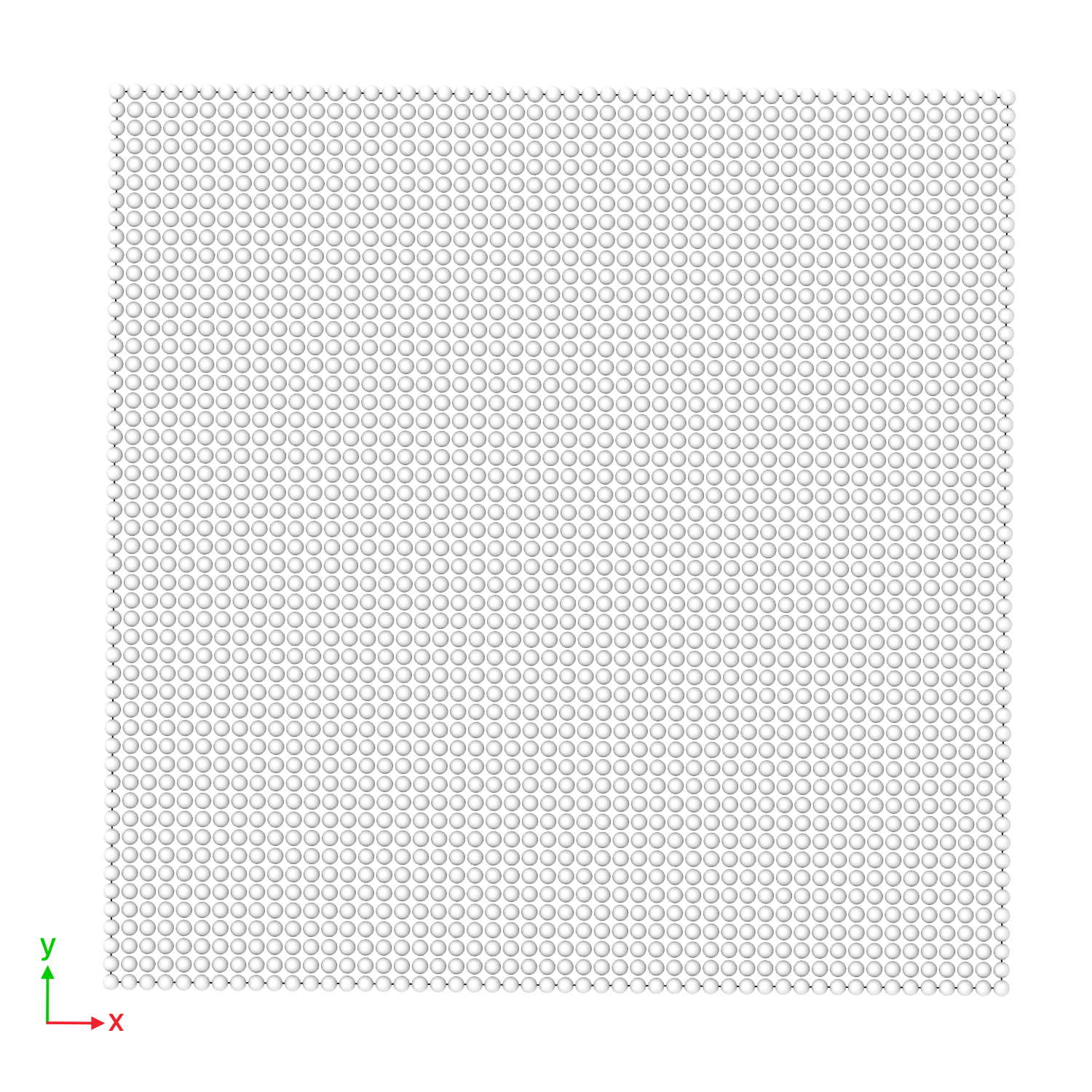
(Right) 2D soft-disk fluid initial state, and (Left) its trajectory
- simplified to demonstrates the core MD loop
- force calculation
- numerical integration of Newton’s equations
- property measurement
- other fundamental concepts
- periodic boundary conditions
- wraparound effect must be considered in both integration of the equations of motion and the interaction computations
- after each integration step the coordinates must be examined
- wraparound effect must be considered in both integration of the equations of motion and the interaction computations
- use of dimensionless units for generality
- generation of initial state
- c++ program
- code: Chapter 2
- constructued incrementally, with most case studies building on programs introduced earlier
- aim is to provide a more general framework that will be utilized later
- periodic boundary conditions
chapter 3
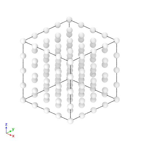
(Right) 3D LJ system initial state, and (Left) its trajectory
- molecules representation:
- atoms with orientation-dependent forces
- extended structures, containing several interaction sites
- rigid, flexible, or in between
- here, it upgrades its components to a more physically realistic model
- simple sof-disk potential replaced by the Lennard-Jones (LJ) potential
- used for liquid argon
- used as a generic potential for qualitative explorations not involving specific substance
- workhorse model for simple fluid that includes both a short-range repulsive term ($r^{-12}$) and a longer-range attractive term ($r^{-6}$)
- details of interaction computation: explaining the necessity of a potential cutoff radius to manage computational cost and the implementation of neighbor lists to avoid redundant force calculations
- typical cutoff: $r_c = 2.5$ (MD units)
- alternative potentials for use in simple cases: replace $r^{-12}$ -> $Ae^{\alpha r}$
- produces a softer central core, but the repulsive part contributes over a longer range
- Cell division method used
- scan over cells, then over offsets and only over cell contents
- heart of the simulation: the numerical integration of the equations of motion
- recipes for and analysis of different algorithms: Verlet leapfrog, predictor-corrector methods
- examines their performance in terms of:
- stability
- long-term energy conservation
- examines their performance in terms of:
- recipes for and analysis of different algorithms: Verlet leapfrog, predictor-corrector methods
- trajectory sensitivity: the inherent chaotic nature of these N-body problems and its implications for reproducibility
- c++ program
- code: Chapter 3
- simple sof-disk potential replaced by the Lennard-Jones (LJ) potential
chapter 4:
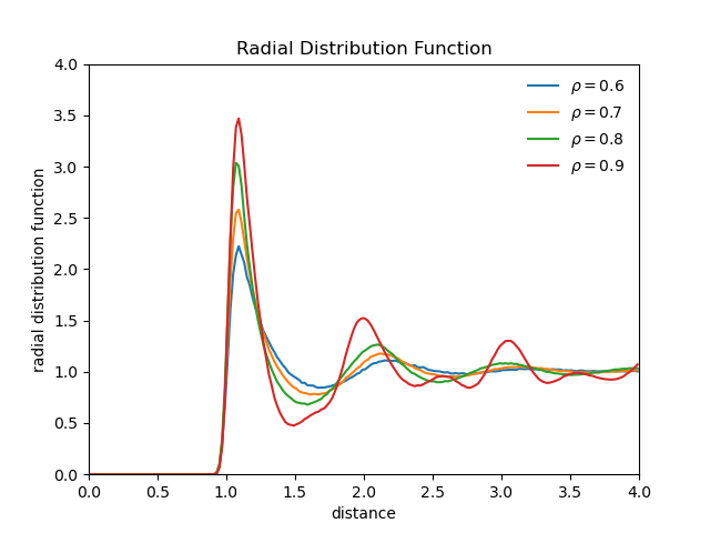
Radial distribution function of a soft-sphere system
- with a robust simulation engine for a realistic fluid in hand, the subsequent chapters focus on how to use it as a numerical “experiment” to make measurements
- equilibrium properties of simple fluids: details the measurement of fundamental quantities
- temperature
- pressure (via virial theorem)
- energy
- spatial structure and organization
- radial distribution function
- doesnt provide information whether a long-range crystalline order exists
- long-range crystalline order corresponds to the presence of a lattice structure
- doesnt provide information whether a long-range crystalline order exists
- long-range crystalline order
- radial distribution function
- equilibrium properties of simple fluids: details the measurement of fundamental quantities
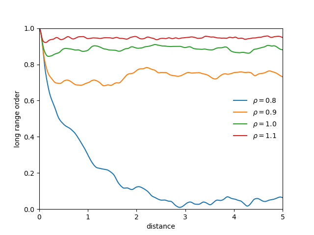
3D soft-sphere system with density of (left) 0.8, and (center) 1.1, (right) and the corresponding long range order
- a test for the presence of long-range order: $|\rho(\mathbf{k})|$
\begin{equation}
\rho(\mathbf{r}) \rightarrow \rho(\mathbf{k}) = \frac{1}{N_m} \sum_{j=1}^{N_m} e^{-i\mathbf{k}\cdot \mathbf{r_j}}
\end{equation}
- using the following expression: $|e^{-i\mathbf{k}\cdot\mathbf{r}_j}| = \sqrt{\cos^2(\mathbf{k}\cdot\mathbf{r}_j)+(-\sin(\mathbf{k}\cdot\mathbf{r}_j))^2}$ , and the definition of the wave vector $\mathbf{k} = 2\pi/l (1, -1, 1)$, where $l$ is the unit cell edge:
- also introduces techniques like cluster analysis for identifying aggregates of particles.
\begin{aligned} |\rho(\mathbf{k})| &= \sqrt{\frac{1}{N_m} \sum_{j=1}^{N_m} e^{-i\mathbf{k}\cdot \mathbf{r_j}}}\\&= \frac{1}{N_m} \sqrt{\sum_{j=1}^{N_m} \cos^2(\mathbf{k}\cdot\mathbf{r_j})+(-\sin(\mathbf{k} \cdot \mathbf{r_j}))^2} \end{aligned}
- code equivalent:
      kVec.x = 2. * M_PI * initUcell.x / region.x;
      kVec.y = - kVec.x;
      kVec.z = kVec.x;
      sr = 0.;
      si = 0.;
      DO_MOL {
          t = VDot (kVec, mol[n].r);
          sr += cos (t);
          si += sin (t);
      }
      latticeCorr = sqrt (Sqr (sr) + Sqr (si)) / nMol;
chapter 5
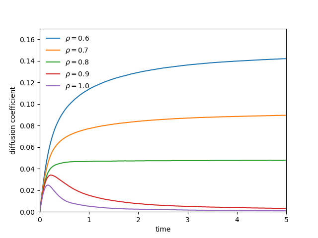
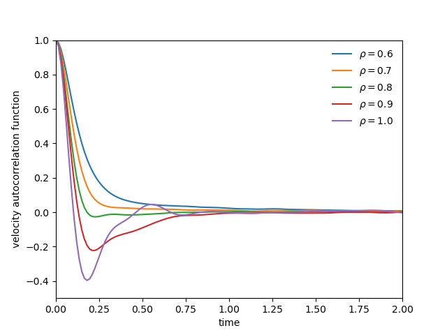
(left) Diffusion coefficient of a soft-sphere system at various density at T=1.0. (right) Velocity autocorrelation function at various density at T=1.0
- dynamical properties of simple fluids: from static snapshots to the time-evolution of the system, explains how to measure transport coefficients
- transport coefficient: material properties of fluid within the framework of continuum fluid dynamics
- can be directly derived from one of the continuum equations of fluid dynamics, such as the Navier-Stokes equation, after taking the long wavelength limit of the Fourier transformed version of the equation
- the constant factor relating the response of a system to an imposed driving force, e.g. Newtonian definition of shear viscosity, or Fourier’s law of heat transport, implies a nonequilibrium system
- diffusion coefficients
\begin{equation}
D = \lim_{t\rightarrow \infty} \frac{1}{6 N_m t} \left\langle \sum_{j=1}^{N_m} \left[ \mathbf{r_j}(t) - \mathbf{r_j}(0)\right]^2\right\rangle
\end{equation}
... DO_MOL { VSub (dr, tBuf[nb].rTrue[n], mol[n].r); VDiv (dr, dr, region); dr.x = Nint (dr.x); dr.y = Nint (dr.y);dr.z = Nint (dr.z); VMul (dr, dr, region); VAdd (tBuf[nb].rTrue[n], mol[n].r, dr); VSub (dr, tBuf[nb].rTrue[n], tBuf[nb].orgR[n]); tBuf[nb].rrDiffuse[ni] += VLenSq (dr); } ... - shear viscosity
- thermal conductivity
- concept of space-time correlation functions is introduced
- linear response theory: describes the reaction of an equilibrium system to a small external perturbation and defines generalized ‘susceptibilities’ that are expressed in terms of various equilibrium correlation functions
- integrating velocity autocorrelation function via the Green-Kubo relations
- transport coefficient: material properties of fluid within the framework of continuum fluid dynamics
- space-time correlation functions
Molecular Modeling and Constraints (6-11)
chapter 6
- The basic MD algorithm naturally simulates the microcanonical (NVE) ensemble, where the number of particles (N), volume (V), and energy (E) are conserved. While fundamental, this does not always match real-world experimental conditions.
- provides the crucial recipes for simulating in more useful statistical ensembles
- details the implementation:
- thermostats (e.g., Berendsen velocity rescaling, Nosé-Hoover) to control temperature for NVT simulations
- barostats to control pressure for NPT simulations.
- Both feedback-based and more rigorous constraint-based methods are explained.
- details the implementation:
- MD is regarded as a tool for generating equilibrium states satisfying certain specified requirements
- no physical meaning is attributed to the actual dynamics, and the approach is merely one of computational convenience for generating particular equilibrium thermodynamics states
- MD vs experimental setupt
- energy and volume are fixed rather than temperature and pressure
- MD: is NVE (microcanonical ensemble)
- experiments: is NVT (canonical ensemble)
- if constant pressure is imposed, as the case in lab : NPT (isothermal-isobaric) ensemble
- modifying the dynamics allows MD to model the equilibrium behaviour of other ensembles directly
- 2 different approach
- use a feedback mechanism for correcting deviations in the controlled parameter from the preset mean value; the value fluctuates, but the size of the fluctuations can be regulated
- rests on the idea that: temperature is proportional to the mean-square velocity it ought to be possible to vary the temperature by adjusting the rate at which time progresses
- new dynamical variable is introduced into the Lagrangian in manner that is equivalent to rescaling the unit of time, and extra terms are added in just the way need to obtain the desired behavior
- two distinct time: real/physical time $t’$, scaled/virtual time ‘t’
- equation of motion resembles conventional Newtonian equation with additional frictionlike term
- a feedback mechanism equation is also obtained from the extended Lagrangian
- the new variable $s$ is varied to regulate the temperature
- pressure can be adjusted by altering the container volume
- a uniform istropic volume change brought about by rescaling the atomic coordinates
- combined with temperature feedback -> isothermal-isobaric (NPT) ensemble
- a uniform istropic volume change brought about by rescaling the atomic coordinates
- augment the equations of motion with suitable mechanical constraints; thus temperature can be held constant by introducing a constraint that fixes the kinetic energy
- use a feedback mechanism for correcting deviations in the controlled parameter from the preset mean value; the value fluctuates, but the size of the fluctuations can be regulated
- other methods
- coupling the system to a constant-temperature heat bath, or even by simply resetting the kinetic energy at each timestep
chapter 7
- takes the next step by showing how to actively drive a system away from equilibrium to measure its response
- provides practical algorithms for simulating phenomena like shear flow to calculate viscosity and for applying thermal gradients to measure thermal conductivity
chapter 8
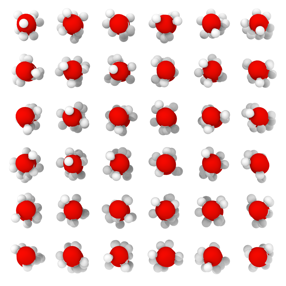
Initial configuration and trajectory of the water molecules of the simulation (T=3.8 in reduced units)
- introduces techniques for simulating molecules where the internal geometry (bond lengths and angles) is held fixed.
- molecules constructed from a rigidly linked atomic framework: the model does not account for chemical processes - no mechanism is provided for molecular formation and dissociation
- classical Euler angles play a central part->quaternions is actually a better choice, dynamics will be described using such quantities
- a common and efficient approach for modeling small, stiff molecules like water.
- provides a case study of a TIP4P-like water mode
-
explains in detail the use of quaternions to describe the orientation and integrate the rotational equations of motion - a non-trivial mathematical and programming challenge
- interactions between rigid molecules are usually expressed as sums of contributions from pairs of interaction sites on different molecules
- it is sufficient to know the center of mass separation of the two molecules and their orientations in order to be able to compute the interactions between the site pairs
- types of measurement
- site-site RDFs
- rotational diffusion: a measure of the rate at which the direction of the molecular dipole changes
- translation diffusion: measured based on the molecular center of mass coordinates
- hydrogen bonds: each molecule forms four strong, highly directional bonds with its immediate neighbors
- basic requirements of any water model is that it should reproduce this behavior
- code: evaluate the interaction energy of each pair of molecules and construct a histogram of these values
- compute the average pair-energy distribution over a series of configurations,
- constructs a histogram of the number of bonds per molecule and outputs the result
chapter 9
- addresses the opposite extreme: fully flexible molecules where bonds can stretch, bend, and twist
- polymers and surfactants
- covers the simulation of a:
- single polymer chain in a solvent
- the fascinating processes of surfactant self-assembly, where amphiphilic molecules spontaneously form structures like micelles in solution
chapter 10
- “geometrically constrained molecule” is important in modern simulation
- details constraint algorithms:
- SHAKE, its velocity-version RATTLE
- used to fix bond lengths and/or angles while allowing other degrees of freedom (like dihedral rotations) to evolve freely
- its a critcal technique that allows for a significantly larger integration timestep, making long simulation feasible
- SHAKE, its velocity-version RATTLE
- primary case study is a “united-atom” model of alkane chains, where CH2 and CH3 groups are treated as single interaction sites.
- details constraint algorithms:
chapter 11
- presents a powerful but more complex alternative. Instead of simulating in Cartesian coordinates and then applying constraints, this approach formulates the equations of motion directly in terms of the system’s true physical degrees of freedom (e.g., bond angles and dihedrals)
- can be a highly efficient method for specific classes of problems, such as modeling long polymer chains.
Advanced Topics and Computational Frontiers (12-18)
MD Programming
- guide the reader from the abstract concept of simulation to the execution and analysis of a working model with efficiency
- chapter 2 code focus: 2D system
- allow the gradual introduction of data structures and other elements that will be used throughtout the book
- new kind of floating-point variable:
real-> single/double precision- single precision saves storeage
- double precision adds accuracy
typedef double real; - speed depends on hardware
- atomic coordinates -> vectors -> atom/molecule
- useful data structure, uses
structto group variables of different types under a single name:typedef struct{ real x, y, z; // 3D // real x, y; // 2D } VecR; typedef struct { int x, y, z; } VecI; typedef struct { VecR r, rv, ra // position, velocity, acceleration } Mol; typedef struct { real val, sum, sum2; } Prop;
- useful data structure, uses
- Memory Allocation:
  #define AllocMem(a, n, t) a = (t *) malloc ((n) * sizeof (t))

  void AllocArrays ()
  {
      // mol = (Mol *)malloc(nMol * sizeof(Mol));
      AllocMem(mol, nMol, Mol);
      // allocation of the histogram
      AllocMem(histVel, sizeHistVel, real);
      // linked list
      AllocMem(cellList, VProd(initUcell) + nMol, int);
      AllocMem(nebrTab, 2 * nebrTabMax, int);
  }
- new kind of floating-point variable:
- useful (annoying) MACRO for vector and scalar manipulation/operation:
- several vector operations are defined:
- vector addition:
VAdd - vector subtraction:
VSub - dot product:
VDot - vector multiplication:
VMul(element wise)
- vector addition:
- other operations:
- vector-scalar:
VSAdd,VVSAdd VSet,VSetAll- initialization to zero:
VZero - vector length:
VLenSq - scaling vector:
VScale
- vector-scalar:
- several vector operations are defined:
- allow the gradual introduction of data structures and other elements that will be used throughtout the book
- NOTE!!!: if the program happens to be called
md_progthen the data file should be namedmd_prog.in