home physics math coding

Two-electron SCF Fortran Code

Started: 02 Aug 2025
Updated: 05 Aug 2025

Table of Content

Table of Content

Main Program

code repo: https://github.com/antble/modernquantumchemistry

two-electron SCF fortran code diagram

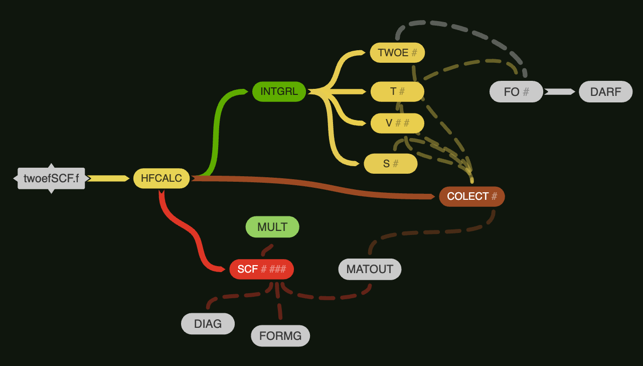
HF Calculation

	IMPLICIT DOUBLE PRECISION(A-H, O-Z)
	IOP = 2 
	N = 3 
	R = 1.4632D0
	ZETA1 = 2.0925D0
	ZETA2 = 1.24D0
	ZA = 2.0D0
	ZB = 1.0D0
	! Call the subroutine to perform the calculation
	CALL HFCALC(IOP, N, R, ZETA1, ZETA2, ZA, ZB)
	END 

	SUBROUTINE HFCALC(IOP, N, R, ZETA1, ZETA2, ZA, ZB)
	IMPLICIT DOUBLE PRECISION (A-H,O-Z)
	IF (IOP .EQ. 0) GOTO 20
	PRINT 10, N, ZA, ZB
10    FORMAT(1H1, 2X, 4HSTO-, I1,21HG FOR ATOMIC NUMBERS, 
     +       F5.2, 5H AND, F5.2)
	 CALL INTGRL(IOP, N, R, ZETA1, ZETA2, ZA, ZB) ! calculate integrals
	 CALL COLECT(IOP, N, R, ZETA1, ZETA2, ZA, ZB) ! put all integrals into arrays
	 CALL SCF(IOP, N, R, ZETA1, ZETA2, ZA, ZB) ! perform SCF calculation
20    CONTINUE
	RETURN
	END

Integral

SCF requires the evaluation of several integrals over the basis set $\{\phi_{\mu} \}$:

$S_{\mu\nu}$
$H_{\mu\nu}^{core} = T + \sum_{i}V_{i}$
two-electron integral ($\mu \nu \mid \lambda \sigma$)

Overlap Integral

overal integral has off-diagonal element calculated using equation (\ref{eq:1}):
- see equation 3.228 in chapter 3 of the book for the derivation
- this quantifies the degree to which the two atomic orbitals share the same space: \begin{equation} S_{\mu \nu} = \sum_{p=1}^{3} \sum_{q=1}^{L} d_{p\mu}^{*} d_{q\nu} S_{pq} \label{eq:1} \quad \mu, \nu = 1,2 \end{equation}
```
...
S12 = S12 + S(A1(I), A2(J), R2)*D1(I)*D2(J) 
...
```
$S_{pq}$ is defined: \begin{equation} S_{pq} = \int d\mathbf{r} \phi_{p}^{GF}(\alpha_{p\mu}, r-R_A)\phi_{q}^{GF}(\alpha_{q\nu}, r-R_B) \end{equation}
- this has analytical solution given in S(A,B,RAB2) function.
final overlap matrix has the form: $S=\left(\begin{array}{cc} 1 & S_{12} \\ S_{12} & 1 \end{array}\right)$

Core Hamiltonian

Kinetic Energy Integral

kinetic integral elements calculated using equation (\ref{eq:2}): \begin{equation} T_{\mu \nu} = \sum_{p=1}^{3} \sum_{q=1}^{L} d_{p\mu}^{*} d_{q\nu} T_{pq} \label{eq:2} \quad \mu, \nu = 1,2 \end{equation}
```
...
T11 = T11 + T(A1(I), A1(J),0.0D0)*D1(I)*D1(J)
T12 = T12 + T(A1(I), A2(J),R2)*D1(I)*D2(J)
T22 = T22 + T(A2(I), A2(J),0.0D0)*D2(I)*D2(J)
...
```
$T_{pq}$ is defined: \begin{equation} T_{pq} = \int d\mathbf{r} \phi_{p}^{GF}(\alpha_{p\mu}, r-R_A)\left[ -\frac{1}{2}\nabla_r^2 \right]\phi_{q}^{GF}(\alpha_{q\nu}, r-R_B) \end{equation}
- this has analytical solution calculated in T(A,B,RAB2) function based on equation \ref{eq:kinsolution}
final kinetic energy matrix has the form, defining the core Hamiltonian matrix:
- represents the total energy of a single electron in the potential of the nuclei, before considering electron-electron repulsion $T=\left(\begin{array}{cc} T_{11} & T_{12} \\ T_{12} & T_{22} \end{array}\right)$

Potential Integral

general formulat for a potential energy integral, representing the attraction of an electron distribution to a nucleus C: \begin{equation} V_{\mu \nu, C} = \sum_{p=1}^{3} \sum_{q=1}^{L} d_{p\mu}^{*} d_{q\nu} V_{pq} \label{eq:3} \quad \mu, \nu = 1,2 \end{equation}
- attraction of an electron in one orbital to the other nucleus ($V_{12}, V_{21}$)
- attraction of an electron to its own nucleus ($V_{11},V_{22}$)
```
DO 20 I=1,N
DO 20 J=1,N
...
V11A = V11A + V(A1(I), A1(J), 0.0D0, 0.0D0, ZA)*D1(I)*D1(J) 
V12A = V12A + V(A1(I), A2(J), R2, RAP2, ZA)*D1(I)*D2(J)
V22A = V22A + V(A2(I), A2(J), 0.0D0, R2, ZA)*D2(I)*D2(J)
V11B = V11B + V(A1(I), A1(J), 0.0D0, R2, ZB)*D1(I)*D1(J)
V12B = V12B + V(A1(I), A2(J), R2, RBP2, ZB)*D1(I)*D2(J)
V22B = V22B + V(A2(I), A2(J), 0.0D0, 0.0D0, ZB)*D2(I)*D2(J)
...
```
- $V_{pq}$ is defined: \begin{equation} V \rightarrow V_{pq} = \int d\mathbf{r} \phi_{p}^{GF}(\alpha_{p\mu}, r-R_A)\left[ -\frac{Z_c}{|r-R_C|} \right]\phi_{q}^{GF}(\alpha_{q\nu}, r-R_B) \end{equation}
  - solution of this is given in equation (\ref{eq:potsolution}), calculated using V(A,B,RAB2,RCP2,ZC) function
  - these potential energy integrals are combined with the kinetic energy integrals to form the core Hamiltonian matrix with elements $H_{\mu\nu}^{core}$

Two-electron Integral Derivation

two-electron integrals are used for computing the $G$ matrix (see FORMG subroutine)
- it accounts for the average repulsion an electron feels from all other electrons
- without this terms, the model incorrectly treat all electrons as independent particles, ignoring the fundamental repulsive forces between them
a set of two-electron integrals (from equation 3.155 of the book): \begin{equation} (\mu\nu\mid\lambda\sigma) = \int d\mathbf{r_1}d\mathbf{r_2} \phi_{\mu}^{*}(1)\phi_{\nu}(1)\frac{1}{r_{12}} \phi_{\lambda}^{*}(2)\phi_{\sigma}(2) \label{eq:twoe} \end{equation}

expanding this equation in the contracted Gaussian and evaluation of the resulting integral gives us: \begin{equation} (\mu \nu \mid \lambda \sigma)=\sum_{i=1}^N \sum_{j=1}^N \sum_{k=1}^N \sum_{l=1}^N d_{\mu, i} d_{\nu, j} d_{\lambda, k} d_{\sigma, l}\left(g_i g_j \mid g_k g_l\right) \end{equation}

computational equivalent:

DO 30 I=1,N
DO 30 J=1,N
DO 30 K=1,N
DO 30 L=1,N
...
    V1111 = V1111 + TWOE(A1(I),A1(J),A1(K),A1(L),0.0D0,0.0D0,0.0D0)
    + *D1(I)*D1(J)*D1(K)*D1(L)
    V2111 = V2111 + TWOE(A2(I),A1(J),A1(K),A1(L),R2,0.0D0,RAP2)
    + *D2(I)*D1(J)*D1(K)*D1(L)
    V2121 = V2121 + TWOE(A2(I),A1(J),A2(K),A1(L),R2,R2,RPQ2)
    + *D2(I)*D1(J)*D2(K)*D1(L)
    V2211 = V2211 + TWOE(A2(I),A2(J),A1(K),A1(L),0.0D0,0.0D0,R2)
    + *D2(I)*D2(J)*D1(K)*D1(L)
    V2221 = V2221 + TWOE(A2(I),A2(J),A2(K),A1(L),0.0D0,R2,RBQ2)
    + *D2(I)*D2(J)*D2(K)*D1(L)
    V2222 = V2222 + TWOE(A2(I),A2(J),A2(K),A2(L),0.0D0,0.0D0,0.0D0)
    + *D2(I)*D2(J)*D2(K)*D2(L)
...

$g_i$ is the primitive Gaussians where solution of such integrals are derived in Appendix A of the book
computation is given by the TWOE(A, B, C, D, RAB2, RCD2, RPQ2) function

Electron Repulsion G matrix

after obtaining the core Hamiltonina, next is to calculate the two-electron part of the Fock Matrix $G_{\mu\nu}$ \begin{equation} F_{\mu\nu } = H_{\mu\nu}^{core} + G_{\mu\nu} \end{equation}
- depends on the density matrix $\mathbf{P}$ and the set of two-electron integrals $(\mu\nu\mid\lambda\sigma)$ (see equation \ref{eq:twoe})
- $\mathbf{G}$ matrix: $\begin{equation} \begin{split} G_{\mu\nu} &= 2\sum_{a}^{N/2} \sum_{\lambda \sigma} C_{\lambda a}C_{\sigma a}^{*}[(\mu\nu\mid\sigma\lambda) - \frac{1}{2} (\mu\lambda\mid\sigma\nu)] \\ &= \sum_{\lambda \sigma} P_{\lambda \sigma}[(\mu\nu\mid\sigma\lambda) - \frac{1}{2} (\mu\lambda\mid\sigma\nu)] \end{split} \label{eq:gmatrix} \end{equation}$
```
DO 10, K=1,2
DO 10, L=1,2
G(I,J) = G(I,J) + P(K,L)*(TT(I,J,K,L)-0.5D0*TT(I,L,K,J))
```
density matrix/charge-density bond-order matrix is defined as: \begin{equation} P_{\lambda \sigma} = 2\sum_{a}^{N/2} C_{\lambda a}C_{\sigma a}^{*} \label{eq:densitymat} \end{equation}
- how do we compute the density matrix $\mathbf{P}$??
  - first is an initial guess, then use SCF procedure to update its value

Collecting the elements

COLECT subroutine purpose is to form the relevant matrices for SCF:
- $\mathbf{S}, \mathbf{H}, \mathbf{X}, X^{\dagger}$, and two-electron integral $(\mu\nu\mid\lambda\sigma)$

overlap matrix, $\mathbf{S}$:

  S(1,1) = 1.0D0
  S(1,2) = S12
  S(2,1) = S(1,2)
  S(2,2) = 1.0D0

core Hamiltonian, $\mathbf{H}$:

  H(1,1) = T11 + V11A + V11B
  H(1,2) = T12 + V12A + V12B
  H(2,1) = T12 + V12A + V12B
  H(2,2) = T22 + V22A + V22B

transformation matrix, $\mathbf{X}$, $\mathbf{X^{\dagger}}$:

  ! use canonical orthogonalization to form the X matrix
  X(1,1) = 1.0D0/DSQRT(2.0D0*(1.0D0 + S12))
  X(1,2) = X(1,1)
  X(2,1) = 1.0D0/DSQRT(2.0D0*(1.0D0 - S12))
  X(2,2) = -X(1, 2)
  ! form the X transpose matrix
  XT(1,1) = X(1,1)
  XT(1,2) = X(2,1)
  XT(2,1) = X(1,2)
  XT(2,2) = X(2,2)

two-electron integral matrix, $(\mu\nu\mid\lambda\sigma)$:

  TT(1,1,1,1) = V1111
  TT(2,1,1,1) = V2111
  TT(1,2,1,1) = V2111
  TT(1,1,2,1) = V2111
  TT(1,1,1,2) = V2111
  TT(2,1,2,1) = V2121
  TT(1,2,2,1) = V2121
  TT(2,1,1,2) = V2121
  TT(1,2,1,2) = V2121
  TT(2,2,1,1) = V2211
  TT(1,1,2,2) = V2211
  TT(2,2,2,1) = V2221
  TT(2,2,1,2) = V2221
  TT(2,1,2,2) = V2221
  TT(1,2,2,2) = V2221
  TT(2,2,2,2) = V2222

Self-Consistent Field (SCF) Procedure

algorithm of the SCF (page 146 of the book), code snippet are from SCF subroutine.
1. diagonalize the overlap matrix S and obtain a transformation matrix X from symmetric orthogonalization: $\mathbf{X} \equiv \mathbf{S}^{-1/2} $
2. obtain a guess at the density matrix $\mathbf{P}$
3. calculate the matrix $\mathbf{G}$ of equation (\ref{eq:gmatrix}) from the density matrix $P$ and the two-electron integrals $(\mu\nu\mid\lambda\sigma)$
4. Add $\mathbf{G}$ to the core-Hamiltonian to obtain the Fock matrix $\mathbf{F}=\mathbf{H}^{core} + \mathbf{G}$
```
  DO 60 I=1,2
  DO 60 J=1,2
  F(I,J) = H(I,J) + G(I,J)
```
5. Calculate the transformed matrix $\mathbf{F’}=\mathbf{X^{\dagger}FX}$
```
  CALL MULT(F,X,G,2,2)
  CALL MULT(XT,G,FPRIME,2,2)
```
6. Diagonalize $\mathbf{F’}$ to obtain $\mathbf{C’}$ and $\epsilon$
```
  CALL DIAG(FPRIME,CPRIME,E)
```
7. Calculate $\mathbf{C=XC’}$
```
  CALL MULT(X,CPRIME,C,2,2)
```
8. form a new density matrix $\mathbf{P}_{new}$ from $\mathbf{C}$ using equation (\ref{eq:densitymat}): $\mathbf{P}\rightarrow \mathbf{P}_{old}, \mathbf{P}_{new} \rightarrow \mathbf{P}$
```
  DO 100 I=1,2
  DO 100 J=1,2
  OLDP(I,J) = P(I,J)
  P(I,J) = 0.0D0
  DO 100 K=1, 1
  P(I,J) = P(I,J) + 2.0D0*C(I,K)*C(J,K)
```
9. determined whether the procedure has converged: $|\mathbf{P}-\mathbf{P}_{old}| < \text{CRIT} $
```
  DATA CRIT/1.0D-4/
  ...
  DO 120 I=1,2
  DO 120 J=1,2
  DELTA = DELTA + (P(I,J) - OLDP(I,J))**2
  120   CONTINUE
  DELTA = DSQRT(DELTA/4.0D0)
  ...
  IF (DELTA .LT. CRIT) GO TO 160
  IF (ITER .LT. MAXIT) GO TO 20
```
10. if it has converged, use the resulting solution ($\mathbf{C, P, F,..}$) to calculate the expectation values and other quantities of interest
```
  ...
 160   CONTINUE
  ! add nuclear repulsion energy to get the total energy
 ENT = EN + ZA*ZB/R
  ... 
```
  - other expectation values: energy, dipole moment, etc.
  - population analyses

Integral Solutions

Two-Electron Integral

FUNCTION TWOE(A, B, C, D, RAB2, RCD2, RPQ2)
    IMPLICIT DOUBLE PRECISION (A-H,O-Z)
    DATA PI/3.1415926535898D0/
    TWOE=2.0D0*PI**(2.5D0)/((A+B)*(C+D)*DSQRT(A+B+C+D))
    + *F0((A+B)*(C+D)*RPQ2/(A*B+C*D))
    + *DEXP(-A*B*RAB2/(A+B)-C*D*RCD2/(C+D))
    RETURN
END

\[(ab|cd) = \frac{2\pi^{5/2}}{(a+b)(c+d)\sqrt{a+b+c+d}} \times \exp\left(-\frac{ab}{a+b}R_{AB}^2 - \frac{cd}{c+d}R_{CD}^2\right) \times F_0(T)\]

where $ T = \frac{(a+b)(c+d)}{a+b+c+d}R^2_{PQ}$ and $F_0(T)$ is the error function computed using F0(ARG) function.

Overlap Energy

see Appendix A for the derivation: \begin{equation} \left(A | B \right) = \frac{\pi}{(\alpha + \beta)}^{3/2} \exp\left[\frac{-\alpha\beta}{(\alpha + \beta)}|R_{AB}|^2\right] \end{equation} where: $R_{AB} = |R_A -R_B|$

FUNCTION S(A,B,RAB2)
    IMPLICIT DOUBLE PRECISION(A-H, O-Z)
    DATA PI/3.1415926535898D0/
    S = (PI/(A+B))**1.5D0*DEXP(-A*B*RAB2/(A+B))
    RETURN
END

Kinetic Energy

see Appendix A for the derivation: \begin{align} \left(A\left|-\frac{1}{2}\nabla^2\right|B\right) = \frac{\alpha \beta}{(\alpha + \beta)} \ [3 - \frac{2\alpha\beta}{(\alpha + \beta)}|R_{AB}|^2]\left[\frac{\pi}{(\alpha + \beta)}\right]^{3/2}\exp\left[\frac{-\alpha\beta}{(\alpha + \beta)}|R_{AB}|^2\right] \label{eq:kinsolution} \end{align}

FUNCTION T(A,B,RAB2)
IMPLICIT DOUBLE PRECISION(A-H, O-Z)
DATA PI/3.1415926535898D0/
    T=A*B/(A+B)*(3.0D0-2.0D0*A*B*RAB2/(A+B))*(PI/(A+B))**1.5D0
    +    *DEXP(-A*B*RAB2/(A+B))
    RETURN
END

Potential Energy

see Appendix A for the derivation: \begin{equation} \left(A\left|-\frac{Z_C}{r_{1C}}\right|B\right) = \frac{-2\pi}{(\alpha + \beta)}Z_c \exp\left[ \frac{-\alpha \beta}{(\alpha + beta)}|R_A - R_B|^2\right] \times F_0[(\alpha + \beta)|R_p - R_C|^2] \label{eq:potsolution} \end{equation}

FUNCTION V(A,B,RAB2,RCP2,ZC)
    IMPLICIT DOUBLE PRECISION(A-H, O-Z)
    DATA PI/3.1415926535898D0/
    V=2.0D0*PI/(A+B)*FO((A+B)*RCP2)*DEXP(-A*B*RAB2/(A+B))
    V = -V*ZC
    RETURN
END

Diagonalization

subroutine uses the Jacobi rotation method, which for a 2x2 matrix provides an exact, analytical solution. \begin{equation} FC = CE \end{equation}
constructing the eigenvectors $C$

\[C=\left(\begin{array}{cc} \cos \theta & \sin \theta \\ \sin \theta & -\cos \theta \end{array}\right)\]

finding the rotation matrix $\theta$:

\[\theta=\frac{1}{2} \arctan \left(\frac{2 F_{12}}{F_{11}-F_{22}}\right)\]

computing the eigenvalues, which are the diagonal elements of the transformed matrix $E=C^TFC$, code uses the explicit formulas for these elements:

\[\begin{aligned} &E_{11}=F_{11} \cos ^2 \theta+F_{22} \sin ^2 \theta+F_{12} \sin (2 \theta)\\ &E_{22}=F_{11} \sin ^2 \theta+F_{22} \cos ^2 \theta-F_{12} \sin (2 \theta) \end{aligned}\]

SUBROUTINE DIAG(F,C,E)
        IMPLICIT DOUBLE PRECISION(A-H,O-Z)
        DIMENSION F(2,2), C(2,2), E(2,2)
        DATA PI/3.1415926535898D0/
        IF (DABS(F(1,1)-F(2,2)) .GT. 1.0D-20) GO TO 10

        THETA = PI/4.0D0
        GO TO 20
  10    CONTINUE

        THETA = 0.5D0*DATAN(2.0D0*F(1,2)/(F(1,1)-F(2,2)))
  20    CONTINUE
        C(1,1) = DCOS(THETA)
        C(2,1) = DSIN(THETA)
        C(1,2) = DSIN(THETA)
        C(2,2) = -DCOS(THETA)
        E(1,1) = F(1,1)*DCOS(THETA)**2+F(2,2)*DSIN(THETA)**2
     $  +F(1,2)*DSIN(2.0D0*THETA)
        E(2,2) = F(2,2)*DCOS(THETA)**2+F(1,1)*DSIN(THETA)**2
     $  -F(1,2)*DSIN(2.0D0*THETA)
        E(2,1) = 0.0D0
        E(1,2) = 0.0D0

        IF(E(2,2) .GT. E(1,1)) GO TO 30
        TEMP = E(2,2)
        E(2,2) = E(1,1)
        E(1,1) = TEMP
        TEMP = C(1,2)
        C(1,2) = C(1,1)
        C(1,1) = TEMP
        TEMP = C(2,2)
        C(2,2) = C(2,1)
        C(2,1) = TEMP
  30    RETURN
       END

Auxilliary Subroutine, Function

Matrix Multiplication

    SUBROUTINE MULT(A,B,C,IM,M)
        IMPLICIT DOUBLE PRECISION(A-H,O-Z)
        DIMENSION A(IM,IM), B(IM,IM), C(IM,IM)
        DO 10, I=1,M
        DO 10, J=1,M
        C(I,J)=0.0D0
        DO 10 K=1,M
10     C(I,J) = C(I,J) + A(I,K)*B(K,J)
        RETURN
    END

Error Function

    FUNCTION FO(ARG)
        IMPLICIT DOUBLE PRECISION(A-H,O-Z)
        DATA PI/3.1415926535898D0/
        IF (ARG .LT. 1.0D-6) GO TO 10

        FO=DSQRT(PI/ARG)*DARF(DSQRT(ARG))/2.0D0
        GO TO 20

10     FO=1.0D0-ARG/3.0D0
20     CONTINUE
        RETURN
    END

    FUNCTION DARF(ARG)
        IMPLICIT DOUBLE PRECISION(A-H,O-Z)
        DIMENSION A(5)
        DATA P/0.3275911D0/
        DATA A/0.254829592D0, -0.284496736D0,1.421413741D0,
    $   -1.453152027D0,1.061405429D0/
        T=1.0D0/(1.0D0+P*ARG)
        TN = T
        POLY = A(1)*TN
        DO 10 I=2,5
        TN = TN*T
        POLY=POLY + A(I)*TN
10     CONTINUE
        DARF = 1.0D0-POLY*DEXP(-ARG*ARG)
        RETURN
    END